ChatGPT can compare the structure of Shakespeare’s four great tragedies. It can read a Python file and point out the bug. But ask it “what were our team’s OKRs last quarter?” and it has nothing to say. The model has never seen your company wiki, and it knows nothing about events after its training cutoff. When a large language model (LLM) admits it does not know, that is the good case. The more common failure is a confident, plausible-sounding fabrication — what the field calls a hallucination.
Two problems sit underneath this gap: missing domain knowledge and a knowledge cutoff in time. Three approaches try to close it. The user can paste the relevant context into every prompt by hand. The team can retrain the model on company data — fine-tuning. Or the model can stay as it is, with an external knowledge base that gets searched and stitched into the prompt at answer time.
The third option wins on cost, speed, and freshness, and over the past few years it has become the de facto standard. Its name is RAG — Retrieval-Augmented Generation. The sections below cover what RAG is, how it differs from fine-tuning, how the four-stage pipeline works, what makes the embedding layer the heart of the system, where RAG shines, and where it breaks down.
What is RAG? Combining Retrieval and Generation
RAG can be stated in one line:
An architecture that retrieves relevant information from an external knowledge base before the LLM generates an answer, and stitches that information into the prompt.
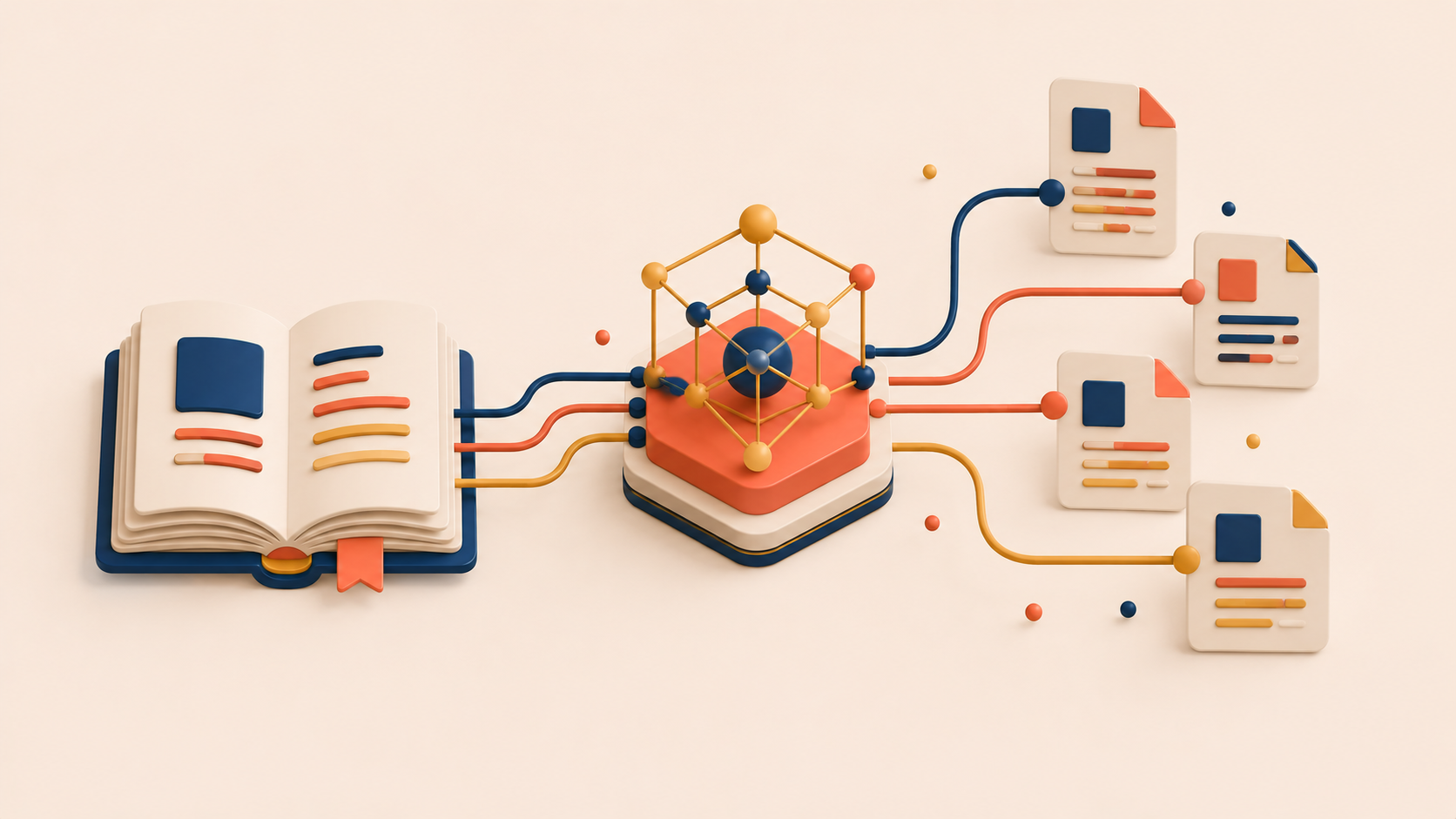
The name says it directly — Retrieval-Augmented Generation. The mental model is an open-book exam. Instead of a student who must answer from memory, picture a student who walks into the exam with the textbook, opens to the right page, and answers from what is on the page.
The open-book pattern fixes four things at once:
- Hallucination drops. The model is not squeezing answers from its own memory; it is reading actual documents and answering from them.
- Post-training information becomes usable. Update the knowledge base and the next answer reflects the update.
- Domain specialization works without retraining. A company wiki, a legal case archive, or a medical guideline can be attached as-is.
- Sources become traceable. The system can mark which document and which chunk produced the answer, which brings trust and auditability.
Patrick Lewis, the first author of the 2020 paper that introduced RAG, has said in interviews that the team was not particularly proud of the name and would have spent more time on it if they had known how widely the term would spread. They could not find anything better before the paper deadline. The acronym we use every day is the result of that deadline.
The biggest reason RAG is attractive is operational: the domain can change without retraining the model. When the knowledge changes, the index is rebuilt. The model stays untouched.
RAG vs Fine-Tuning: Where the Knowledge Lives
A natural question comes up the first time someone meets RAG:
“Why not just retrain the model on our company data?”
That is fine-tuning. Both fine-tuning and RAG share the same goal — letting an LLM act on your data — but they differ in something fundamental.
The difference is where the knowledge lives. Fine-tuning puts the knowledge inside the model. The weights get adjusted so the model itself “remembers” the information. RAG keeps the knowledge outside the model. The model stays as it is, and at answer time, the system fetches external documents and slips them into the prompt.
When knowledge lives inside the model, changing it means retraining. That makes fine-tuning expensive to update and slow to refresh. Correcting a single wrong fact is hard — the information is scattered across the weights, and there is no precise place to edit. Source tracing fails for the same reason. Ask the model where an answer came from, and it cannot point anywhere; the information dissolved into the weights and lost its origin.
When knowledge lives outside the model, the situation flips. Update a document, and the next answer reflects the update. Fix a wrong fact by editing one file. The chunk that produced the answer can be cited directly, because the model received that chunk as input.
When is fine-tuning the right tool, then?
When you want to change behavior, not knowledge. A company’s tone of voice, a consistent output format, a domain-specific reasoning pattern — none of these change when you paste documents into the prompt. They are habits of the model itself, and they have to be trained in. The reverse — “make the LLM aware of our internal manual” — is overwhelmingly a RAG job. Hybrid stacks are common in production (fine-tune for tone, RAG for knowledge), but when the goal is specifically “make the LLM aware of our documents,” the first attempt is almost always RAG.
How RAG Works: The Four-Stage Pipeline
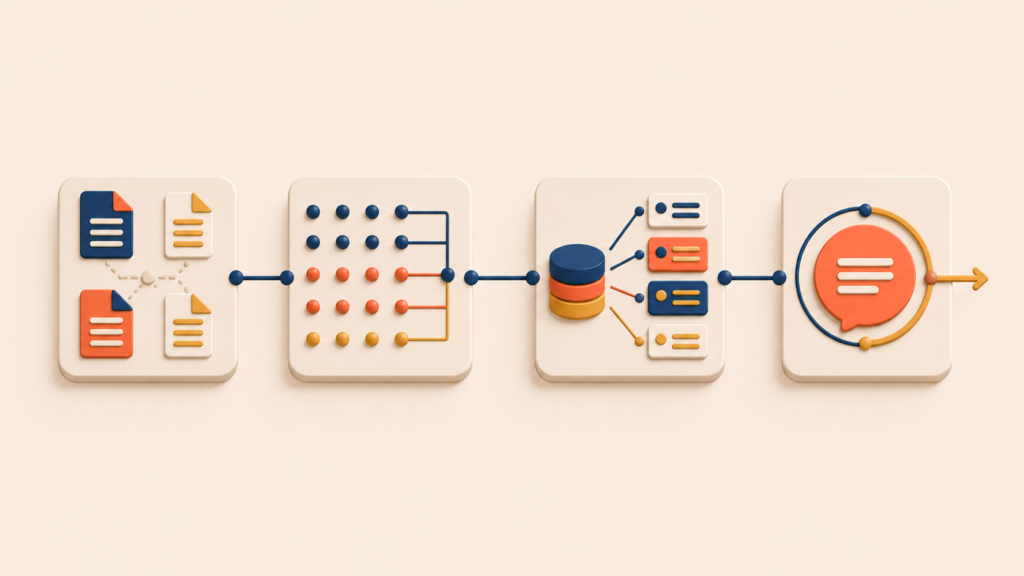
RAG moves through four stages. Understanding the flow makes it clear where the limits show up later.
Stage 1: Indexing (offline). Documents are cut into pieces of reasonable size, called chunks. A chunk might be a paragraph or a few sentences. Each chunk is run through an embedding model, which turns it into a vector — a long list of numbers. The vectors are stored in a vector database. This is the preparation step, done before any user asks anything.
Stage 2: Query embedding. When the user asks a question, the question goes through the same embedding model and becomes a vector. The chunks and the question have to sit in the same coordinate space for comparison to mean anything.
Stage 3: Retrieval. The system searches the vector database for the chunk vectors closest to the question vector. The top N chunks are returned — N is typically 5 to 20.
Stage 4: Generation. The retrieved chunks are inserted into a prompt and sent to the LLM. The prompt usually takes a form like: “Use the following documents to answer the question. [chunk 1] [chunk 2] [chunk 3] / Question: …”. The LLM reads the chunks and produces the answer.
Of the four stages, the one that decides the quality of the product is Stage 3 — retrieval. If retrieval pulls the wrong chunks, the answer falls apart no matter how strong the LLM is. “Garbage in, garbage out” applies here in a very direct way. The next section is where retrieval actually happens.
Inside RAG: Embeddings, Semantic Search, and Vector Databases
RAG retrieval is not keyword search. It runs on semantic similarity. This is the source of RAG’s power, and also the root of the limits that surface later.
Embeddings: turning text into coordinates
Embedding is the operation that converts text into a vector of hundreds or thousands of numbers. Before going further, it helps to be clear about what a vector is.
A vector is a list of numbers. The (x, y) pair you used to mark a point on a coordinate plane in school is a two-dimensional vector. Three dimensions adds z. A 1,536-dimensional vector is a list of 1,536 numbers. Each number describes how far the point sits along one axis of the space.
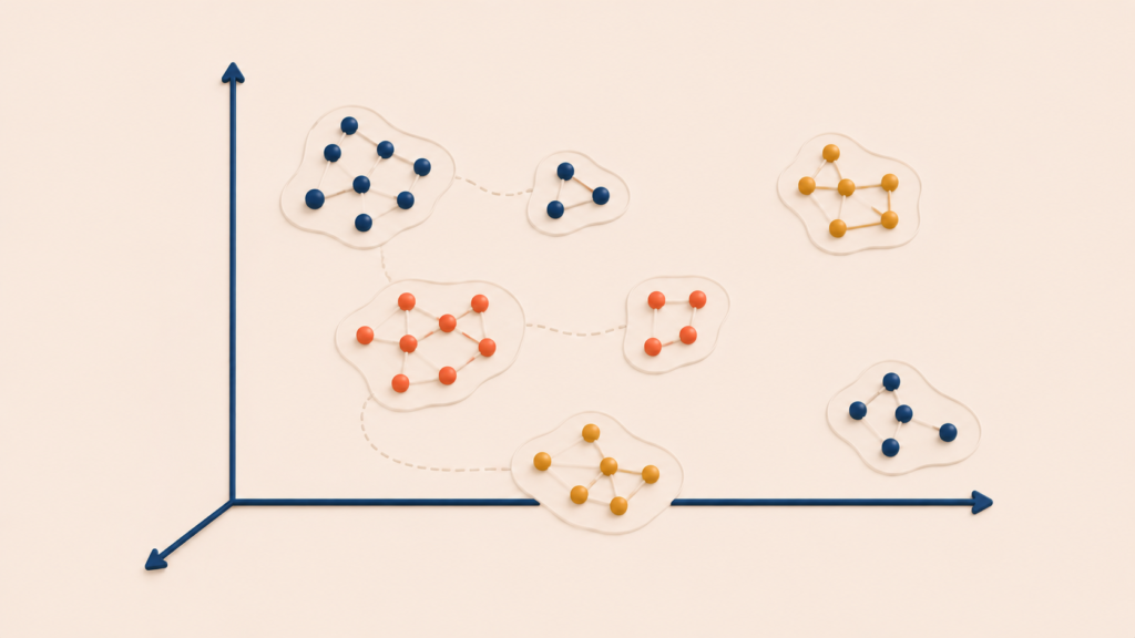
Higher dimensions are impossible to picture, but the math still works. Distances between points can be computed, and “which point is closer to which” can be decided. An embedding turns a piece of text into a single point in this high-dimensional space. Text with similar meaning lands at nearby points; text with different meaning lands far apart.
For example, OpenAI’s text-embedding-3-small produces 1,536-dimensional vectors by default, and text-embedding-3-large goes up to 3,072 dimensions. A 1,536-dimensional embedding means each sentence or chunk is represented by 1,536 numbers.
The dimension count is high because meaning does not collapse to one or two axes. The word “dog” alone carries information about animal type, size, friendliness, responsibility, fur length, the sound it makes, and more. The more dimensions, the better these subtle differences can be captured.
The core property is this: text with similar meaning lands at nearby coordinates. “How to raise a puppy” and “guide to caring for a companion dog” use different words, but their coordinates are close. That is why search works even when the keywords do not match. This is semantic search.
Keyword search vs semantic search
Pure semantic search has weak spots. Exact identifiers like ORD-2024-7821, and domain-specific proper nouns, are two of them. “Puppy” and “companion dog” sit close in vector space, but so do ORD-2024-7821 and ORD-2024-7822 — the embedding cannot read a one-digit difference as a meaningful one. So the cases keyword search handles trivially become semantic search’s blind spots.
Hybrid search fills the gap. It runs vector-based semantic search and keyword search (sparse methods like BM25) in parallel, then fuses the two rankings. Semantic search retrieves pages that mean roughly the same thing; keyword search retrieves pages that contain the exact term; a fusion step scores and combines them into one final ranking. Semantic similarity and lexical match get caught at the same time.
Reciprocal Rank Fusion (RRF) and weighted averaging are common fusion methods. The fusion step is where the system decides how much to trust each signal when the two searches disagree. The weights are tuned per domain — for example, legal text leans on keyword signal, while general FAQ leans on semantic signal.
As of April 2026, most major vector databases support this natively. Weaviate ships BlockMax WAND for accelerated BM25 and offers RankedFusion or RelativeScoreFusion. Milvus 2.5+ generates sparse vectors automatically through a built-in BM25 function. Qdrant uses named vectors to hold dense and sparse vectors side by side. Pinecone exposes a single sparse-dense hybrid index.
What a vector database actually does
A million documents produce several million chunks. Computing the distance between the question vector and every chunk vector for every query would take seconds per answer. For vector search to be practical, a data structure that finds nearby neighbors fast is required.
The vector database is built for exactly this job. The core technique is Approximate Nearest Neighbor (ANN) search. Instead of finding the 100% exact top match, it finds the 99% correct top match in roughly 1/1000 of the time. For a system like RAG — which needs “the top N relevant chunks” rather than “the single mathematically perfect chunk” — trading 1% accuracy for 1000x speed is a clear win.
The most widely used ANN algorithm is HNSW (Hierarchical Navigable Small World). The name is intimidating; the idea is simple. Vectors are stacked in layers, with the upper layers connected sparsely (like highways) and the lower layers densely (like local streets). A query starts at the top, takes the rough direction, then descends layer by layer to zoom in. It is the same shape as flying to a city, taking the subway to a neighborhood, then walking to the actual address.
This is why a vector database is classified not as “a database that holds vectors” but as a search engine indexed for vector retrieval. Adding a vector column to a general RDB does not make RAG run. If retrieval is not fast enough, the user experience collapses. That said, extensions like PostgreSQL’s pgvector add ANN indexes on top of existing databases, and they are a common choice when the data sits below tens of millions of vectors — you keep operational simplicity and get acceptable retrieval performance at the same time.
RAG’s intelligence is, ultimately, the embedding’s intelligence. When the embedding captures meaning well, RAG answers well. When the embedding misses something, RAG misses it too. The vector database fetches what the embedding produced; it does not invent information the embedding failed to encode. This point returns in the final section, where RAG’s limits become concrete.
RAG Use Cases: Where It Shines
Now that the mechanics are clear, the next question is “where is RAG actually worth using?” Four scenarios stand out.
Knowledge bases full of unstructured text. Most of the knowledge that accumulates inside a company is unstructured — PDFs, meeting notes, wikis. Moving that material into a structured database is not practical, and when it is forced, meaning gets lost. RAG makes the content searchable while leaving the documents as they are, which fits the shape of enterprise data well.
Domains where information moves fast. Product changelogs, support articles, regulatory updates, internal policy revisions. The cost of keeping RAG current is the cost of rebuilding an index. Fine-tuning would require retraining for every update.
Domains where source attribution matters. Legal research, medical guidance, financial analysis, internal compliance — any case where the answer has to be checkable. RAG can show which document and which chunk produced an answer; a fine-tuned model cannot.
Customer support and internal search. Both involve a large body of documentation and questions whose answers usually sit inside a single article or a small set of articles. This is where RAG’s retrieval pattern is at its strongest.
Put these four together, and the reason cloud and enterprise providers — AWS, Microsoft, Google, IBM, Oracle — have all built RAG offerings becomes clear. It is the most realistic way to connect internal knowledge to AI, and the cost structure makes operational sense.
Where RAG Breaks Down: Multi-Hop Reasoning and Missing Relationships
So far, RAG sounds close to universal. In production, a pattern shows up that complicates the picture. Simple fact lookups land cleanly. Slightly more complex questions start to wobble. This section is the starting point for the next article.
Researchers have catalogued six recurring weaknesses in RAG. The two most fundamental are multi-hop reasoning and missing relationships. The other four — chunking strategy, metadata enrichment, update pipeline design, and similar operational concerns — can be softened with engineering. The first two cannot, because they are produced by the mechanism of vector similarity itself.
Multi-hop reasoning
A multi-hop question looks something like this:
“Who is A’s direct manager, and what was the average lead time of the projects that manager led last year?”
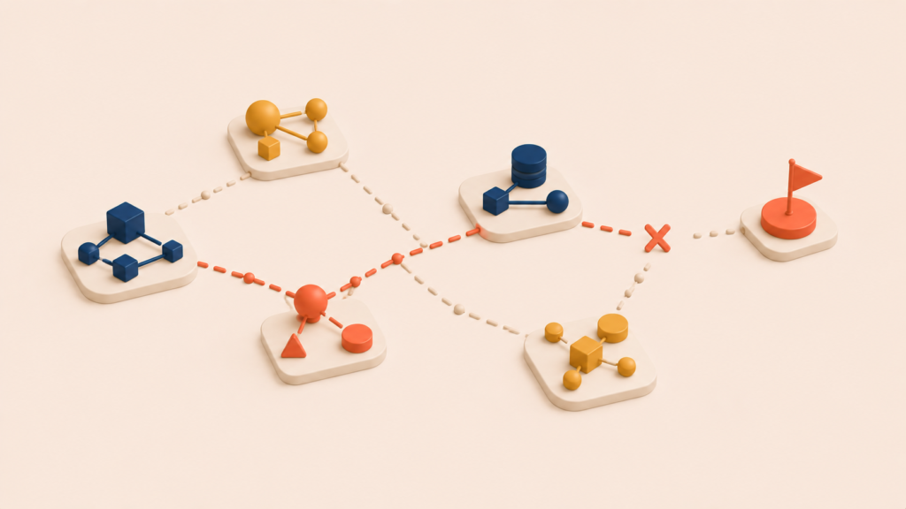
This needs at least three jumps: A → manager → that manager’s projects → the lead time of those projects. If by luck all of this sits in a single chunk, the question resolves. If the information is scattered across documents, RAG cannot assemble it. Even if the first retrieval returns the chunk with “A’s manager,” the standard RAG pipeline has no step that takes the result and runs a second retrieval for “that manager’s projects.”
Missing relationships
The relationship problem runs one level deeper. RAG’s index holds chunks as points scattered in coordinate space — and nothing connects the points. Relationships that exist in the source text in plain language (“this person belongs to that team,” “this incident caused that incident”) survive in the prose but disappear at the index step. The system has to hope the LLM can reconstruct them by reasoning over the retrieved chunks. When chunks are short and the relationships span far, that reconstruction breaks down quickly.
The split between RAG’s wins and RAG’s losses comes down to one question: is the answer contained in a single chunk, or does it require connecting several chunks? A useful image: RAG is a librarian who finds books on similar topics. Even if you do not remember the exact title, the librarian brings you a book on the right subject. What the librarian does not do is tell you how this book relates to that book, or which character connects to which. Those relationships may be written in the books, but they are not in the librarian’s head.
Conclusion
RAG is the open-book exam pattern for LLMs. It takes a model trained on the public internet and gives it access to documents it has never seen, without retraining anything. It reduces hallucination, supports source attribution, and lets a domain change at the speed of an index rebuild instead of the speed of a training run.
The pattern is strong when an answer sits inside a single chunk or a small set of chunks, and the question can be matched on semantic similarity. The pattern weakens when the answer requires traversing relationships across chunks — multi-hop reasoning and the absence of structural links in the index are the two limits that operational tuning cannot fully fix.
The next article picks up exactly where RAG leaves off: how to represent the relationships between chunks at the index level. Knowledge graphs and ontologies are the standard answer to that question, and GraphRAG is the architecture that combines them with retrieval-augmented generation.
RAG Series
(1) What is RAG? Retrieval-Augmented Generation Explained
(2) GraphRAG Explained: Ontology, Knowledge Graphs, and How They Extend RAG
Leave a Reply